
Configuring & Running a Simulation
The Analysis Setup & Run region of the Simulation Dashboard panel is used to configure and run the simulation analyses. Once the circuit is verified and prepared for simulation, configure the required analysis type as described in the below sections.

The Analysis Setup & Run region of the Simulation Dashboard panel
The following sections describe how to configure the common simulation analyses and additional simulation settings.
Operating Point Analysis
The Operating Point analysis is used to determine the DC operating point of a circuit, with inductors shorted and capacitors opened. This analysis calculates the values of current and voltage balance points in a steady-state circuit operation, the transfer coefficients in DC mode, as well as calculating the poles and zeros of the AC transfer characteristic that is required in other types of calculations.
The Operating Point analysis is configured in the Operating Point region of the Simulation Dashboard panel.
Use the Display on schematic buttons to display the calculated values directly on the schematic:
- Voltage – display node voltages in relation to the reference node
- Power – display instant power consumed (positive value) or emitted (negative value)
- Current – display component output current.
After running the analysis, the computed voltage, power, and/or current values will be shown as labels at corresponding nodes.
The simulation result document will include the calculations of the probe placed in the circuit.
An example of a configured Operating Point analysis for a circuit and the simulation result document is shown below. Note that the result value labels (for enabled voltage and power calculations) that appear after the simulation run are shown in the schematic sheet. An example of adding another calculated value to the simulation result document is also shown.


Transfer Function Analysis
The Transfer Function analysis (DC small signal analysis) calculates the DC input resistance, DC output resistance and DC gain, at each voltage node in the circuit.
To perform the Transfer Function analysis, enable the Transfer Function option in the Operating Point region of the Simulation Dashboard panel. Once the option is enabled, the corresponding analysis options are available:
- Source Name – the small signal input source used as the input reference for the calculations.
-
Reference Node – the node in the circuit used as a reference for the calculations at each specified voltage node. '
0' is the reference node (GNDby default).
An example of a configured Transfer Function analysis for a circuit and the simulation result document is shown below. In the simulation result document, select the Transfer Function chart by clicking the tab at the bottom of the design space to access the analysis results.
![]()

Pole-Zero Analysis
The Pole-Zero analysis enables you to determine the stability of a single input, single output linear system, by calculating the poles and/or zeros in the small-signal AC transfer function for the circuit. The DC operating point of the circuit is found and then linearized, small-signal models for all non-linear devices in the circuit are determined. This circuit is then used to find the poles and zeros that satisfy the nominated transfer function.
To perform the Pole-Zero analysis, enable the Pole-Zero Analysis option in the Operating Point region of the Simulation Dashboard panel. Once the option is enabled, the corresponding analysis options are available:
-
Input Node – the positive input node for the circuit.
-
Input Reference Node – the reference node for the input of the circuit.
-
Output Node – the positive output node for the circuit.
-
Output Reference Node – the reference node for the output of the circuit.
-
Analysis Type – allows you to further refine the role of the analysis. Choose to find all poles that satisfy the transfer function for the circuit (
Poles Only), all zeros (Zeros Only), or bothPolesandZeros. -
Transfer Function Type – defines the type of AC small-signal transfer function to be used for the circuit when calculating the poles and/or zeros. There are two types available:
-
V(output)/V(input) – Voltage Gain Transfer Function.
-
V(output)/I(input) – Impedance Transfer Function.
-
An example of a configured Pole-Zero analysis for a circuit and the simulation result document is shown below. In the simulation result document, select the Pole-Zero Analysis chart by clicking the tab at the bottom of the design space to see the analysis results.


DC Sweep
The DC Sweep analysis generates output like that of a curve tracer. It performs a series of Operating Point analyses, modifying the values of selected parameters in pre-defined steps, to give a DC transfer curve.
The DC Sweep analysis is configured in the DC Sweep region of the Simulation Dashboard panel.
Click the Add Parameter control to add the parameters to be stepped. It can be the DC value of a voltage or current source, a resistor value, or temperature (Temp). In the From, To, and Step fields, specify the starting value, the final value, and the incremental value to use over the defined sweep range, respectively.
Use the Output Expressions section to add expressions to be output as waveforms in the simulation result documents (in addition to waveforms for the probes placed in the circuit). Refer to the Adding Output Expressions section to learn more.
An example of a configured DC Sweep analysis for a circuit and the simulation result document is shown below.


Transient
The Transient analysis generates output similar to that normally shown on an oscilloscope, computing the transient output variables (voltage or current) as a function of time, over the user-specified time interval or the number of periods. An Operating Point analysis is automatically performed prior to a Transient analysis to determine the DC bias of the circuit, unless the Use Initial Conditions option is enabled.
The Transient analysis is configured in the Transient region of the Simulation Dashboard panel.
Define the time interval / the number of periods for analysis by selecting the required mode and defining corresponding values:
-
 – Interval mode. Define the value for the start and end of the required time interval (in seconds) and the nominal time increment in the From, To, and Step fields.
-
 – Period mode. Define the value for the start and end of the required time interval (in seconds), the number of periods of a sinusoidal waveform, and the number of data points per sinusoidal waveform period in the From, N Periods, and Points / Period fields.
Use the Output Expressions section to add expressions to be output as waveforms in the simulation result documents (in addition to waveforms for the probes placed in the circuit). Refer to the Adding Output Expressions section to learn more.
Enable the Use Initial Conditions option to use initial conditions to calculate the transient process, bypassing the Operating Point analysis. Use this option when you wish to perform a transient analysis starting from other than the quiescent operating point. The initial condition can be defined for each appropriate component in the schematic (define the value of the corresponding parameter, e.g., Initial Current for an inductor or Initial B-E Voltage or Initial C-E Voltage for a bipolar transistor), or .IC devices can be placed in the circuit (use the Simulate » Place Initial Condition command from the main menus or place the .IC component from the Simulation Generic Components library and then set the Initial Voltage value of the placed component). The IC value of a component overrides an .IC object attached to a net.
An example of a configured Transient analysis for a circuit and the simulation result document is shown below.
![]()
![]()
Fourier Analysis
Fourier analysis of a design is based on the last cycle of transient data captured during a Transient analysis. For example, if the fundamental frequency is 1kHz, then the transient data from the last 1ms cycle would be used for the Fourier analysis.
To perform Fourier analysis, enable the Fourier Analysis option in the Transient region of the Simulation Dashboard panel. Once the option is enabled, the corresponding analysis options are available:
- Fourier Fundamental Frequency – the frequency of the signal that is being approximated by the sum of sinusoidal waveforms.
- Fourier Number of Harmonics – the number of harmonics to be considered in the analysis. Each harmonic is an integer multiple of the fundamental frequency. Together with the fundamental frequency sinusoid, the harmonics sum to form the real waveform of the signal being analyzed. The more harmonics involved in the sum, the greater the approximation to the signal's waveform (e.g., summing sinusoids to form a square wave).
An example of a configured Fourier analysis for a circuit and the simulation result document is shown below. The first two plots show waveforms from the Transient analysis of the circuit, while the subsequent plots that are presented on a separate Fourier Analysis chart of the simulation result document show the results of Fourier analysis. The square wave, whose fundamental frequency is 1kHz, is broken down into sinusoids with frequencies that are odd multiples of this frequency (odd harmonics), as shown in the third plot (1kHz, 3kHz, 5kHz, 7kHz, etc) and with amplitudes that decrease with each subsequent harmonic.

![]()

Stress Analysis
Stress analysis is used to calculate operating conditions for each individual component, such as maximum voltages, currents, and power dissipations, and check them against limits defined in the stress model of the component.
The stress model of a component is configured on the Stress tab of the Sim Model dialog accessed for the component's simulation model. From here, you can select the required Device Type and define parameter values, and also define pin mapping between the stress model (which pins are predefined) and the simulation model. Refer to the Single Component Editing page to learn more about stress analysis model configuration.
Derating coefficients that reduce the parameter limit values are calculated based on the stress model parameters. Alternatively, the values can be set on the Stress tab of the Advanced Analysis Settings dialog (accessed by clicking the Settings control in the Analysis Setup & Run region of the Simulation Dashboard panel).
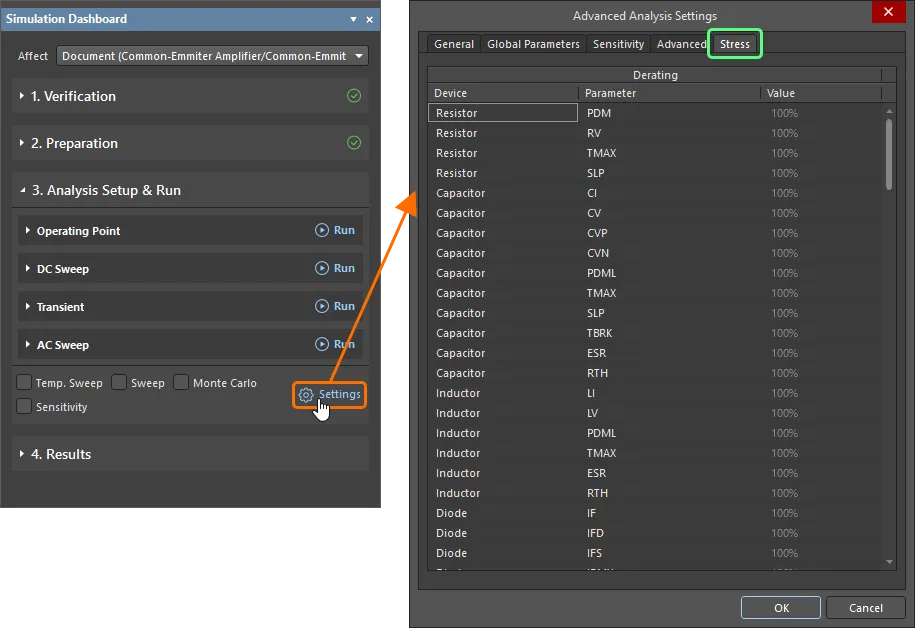
To perform stress analysis, enable the Stress Analysis option in the Transient region of the Simulation Dashboard panel. In the simulation result document, select the Stress chart by clicking the tab at the bottom of the design space to access the analysis results.


AC Sweep
The AC Sweep analysis generates output that shows the frequency response of the circuit, calculating the small-signal AC output variables as a function of frequency. It first performs an Operating Point analysis to determine the DC bias of the circuit, replacing the signal source with a fixed amplitude sine wave generator, then analyzing the circuit over the specified frequency range. The desired output of an AC Small Signal analysis is usually a transfer function (voltage gain, trans-impedance, etc.).

The AC Sweep analysis is configured in the AC Sweep region of the Simulation Dashboard panel.
Define the following parameters for the analysis:
- Start Frequency – the initial frequency for the sine wave generator (in Hz).
- End Frequency – the final frequency for the sine wave generator (in Hz).
- No. Points / Points/Dec / Points/Oct – the incremental value for the sweep range, in conjunction with the chosen Type.
-
Type – the type of data point allocation in the frequency spectrum. The following three types are available:
- Linear – total number of data points evenly spaced on a linear scale.
- Decade – number of evenly spaced data points per decade of a log10 scale.
- Octave – number of evenly spaced data points per octave of a log2 scale.
Use the Output Expressions section to add expressions to be output as waveforms in the simulation result documents (in addition to waveforms for the probes placed in the circuit). Refer to the Adding Output Expressions section to learn more.

An example of a configured AC Sweep analysis for a circuit and the simulation result document is shown below.


Noise Analysis
The Noise analysis measures the noise contributions of resistors and semiconductor devices by plotting the Noise Spectral Density, which is the noise measured in Volts squared per Hertz (V2/Hz). Capacitors, inductors, and controlled sources are treated as noise free.
To perform the Noise analysis, enable the Noise Analysis option in the AC Sweep region of the Simulation Dashboard panel. Once the option is enabled, the corresponding analysis options are available:
-
Noise Source – an independent voltage source in the circuit which is to be used as an input reference for the noise calculations.
-
Output Node – the node in the circuit at which the total output noise is to be measured.
-
Ref Node – the node in the circuit used as a reference for calculating the total output noise at the desired Output Node. By default, this parameter is set to '
0' (the reference node,GNDby default). If set to any other node, the total output noise is calculated asV(Output Node) - V(Reference Node). -
Points Per Summary – allows you to control which noise measurement is performed. The following values of the option are supported:
-
0– setting this parameter to this value will cause input and output noise to be measured only. -
1– setting this parameter to this value will measure the noise contribution of each component in the circuit.
-
An example of a configured Noise analysis for a circuit and the simulation result document is shown below.
In the simulation result document, select the Noise Spectral Density chart by clicking the tab at the bottom of the design space and add the required waves to the current plot by selecting the corresponding entry in the Source Data list in the Sim Data panel and clicking the Add Wave to Plot button. The onoise_spectrum waveform (blue) shows the total output noise measured at the specified output node, in this case Output. The inoise_spectrum waveform (red) shows the amount of noise that would have to be injected at the input to obtain the measured output noise at this node.
Similarly, select the Integrated Noise chart by clicking the tab at the bottom of the design space and add the required calculated values to the results table by selecting the corresponding entry in the Source Data list in the Sim Data panel and clicking the Add Wave to Plot button.


S-Parameters Analysis
S-parameters (scattering parameters) facilitate an approach for describing networks based on the ratio of incident and reflected microwaves (for a device under test, how much power passes from one port to another and how much power is reflected back). These ratios can be subsequently used to calculate properties of a circuit including input impedance, frequency response and isolation. While analysis of S-parameters is primarily for RF circuits and components, it is equally of use to any circuit with at least two sources (ports).
To perform the S-parameters analysis, enable the S-Parameters Analysis option in the AC Sweep region of the Simulation Dashboard panel. Once the option is enabled, the corresponding analysis options are available. Define the ports (sources) involved and set an impedance for each (default is 50 ohms). If a device has more than two ports, these can be added (using the Add control) and defined accordingly, which will result in more S-parameters involved in the resulting ‘S-matrix.’
The simulation engine also calculates Y-parameters (admittance) and Z-parameters (impedance), which can be added to plots in the chart as desired.
Use the Output Expressions section to add expressions to be output as waveforms in the simulation result documents in the form of s_<m>_<n>, y_<m>_<n>, or z_<m>_<n>, for example, s_1_1 or y_1_2.
Once the AC sweep analysis is run, the S-parameters data will be available on the S-parameters Analysis chart in the simulation result document.
An example of a configured S-parameters analysis for a circuit and the simulation result document are shown below.


Additional Analyses
A number of additional analysis types are available. The principle of additional calculations is based on going through the values of the parameters within the selected range and executing a series of calculations for each value of the parameters.
Temperature Sweep
The Temperature Sweep feature is used to analyze the circuit at each temperature in a specified range, producing a series of curves, one for each temperature setting.
To perform the Temperature Sweep analysis, enable the Temp. Sweep option at the bottom of the Analysis Setup & Run region of the Simulation Dashboard panel. Click Settings to configure the analysis in the Temperature region on the General tab of the Advanced Analysis Settings dialog that opens using the following parameters:
- From – the initial temperature of the required sweep range (in Degrees C).
- To – the final temperature of the required sweep range (in Degrees C).
- Step – the incremental step to be used in determining the sweep values across the defined sweep range.
An example of a configured AC Sweep analysis for a circuit in conjunction with the Temperature Sweep feature and the simulation result document is shown below.


Parameter Sweep
The Parameter Sweep feature allows you to sweep the values of devices, sources and/or temperature in defined increments, over a specified range.
To perform the Parameter Sweep analysis, enable the Sweep option at the bottom of the Analysis Setup & Run region of the Simulation Dashboard panel. Click Settings to configure the analysis in the Sweep Parameter region on the General tab of the Advanced Analysis Settings dialog that opens. Click the Add Parameter control to add a parameter to be stepped and select the parameter in the drop-down menu. Select the type of stepped parameter distribution and the fields below to set distribution parameters:
- Linear – specify the starting value, the final value, and the incremental value to use over the defined sweep range in the From, To, and Step fields, respectively.
- Decade – specify the starting value, the final value, and the number of data points by a tenfold order of parameter value change in the From, To, and Points/Dec fields, respectively.
- Octave – specify the starting value, the final value, and the number of data points by a double order of parameter value change in the From, To, and Points/Oct fields, respectively.
- List – specify a list of required parameter values (separated by space) in the Values field.
Add and configure as many parameters to be stepped as needed.
An example of a configured Transient analysis for a circuit in conjunction with the Parameter Sweep feature and the simulation result document is shown below.


Monte Carlo
Monte Carlo analysis allows you to perform multiple simulation runs with component values randomly varied across specified tolerances.
To perform the Monte Carlo analysis, enable the Monte Carlo option at the bottom of the Analysis Setup & Run region of the Simulation Dashboard panel. Click Settings to configure the analysis in the Monte Carlo region on the General tab of the Advanced Analysis Settings dialog that opens using the following parameters:
- Number of Runs – the number of simulation runs you want the simulator to perform. Different device values will be used for each run, within the specified tolerance range. (Default = 5).
-
Distribution – this parameter defines the distribution of values obtained during random number generation. Three distribution types are available:
-
Uniform(Default) – this is a flat distribution. Values are uniformly distributed over the specified tolerance range. For example, for a 1K resistor with a tolerance of 10%, there is an equal chance of the randomly generated value being anywhere between 900Ω and 1100Ω. -
Gaussian– values are distributed according to a Gaussian (bell-shaped) curve, with the center at the nominal value and the specified tolerance at +/- 3 standard deviations. For a resistor with a value of 1K +/- 10%, the center of the distribution would be at 1000Ω, +3 standard deviations is 1100Ω and -3 standard deviations is 990Ω. With this type of distribution, there is a higher probability that the randomly generated value will be closer to the specified value. -
Worst Case– this is the same as the Uniform distribution, but only the end points (worst case) of the range are used. For a 1K +/- 10% resistor, the value used would be randomly chosen from the two worst case values of 990Ω and 1100Ω. On any one simulation run there is an equal chance that the high-end worst case value (1100Ω) or low-end worst case value (990 Ω) will be used.
-
-
Seed – this value is used by the simulator to generate random numbers for the various runs of the analysis. If you want to run a simulation with a different series of random numbers, this value must be changed to another number.
(Default = -1). -
Group Tolerances:
- Resistor – the tolerance to be observed for resistors. The value is entered as a percentage (Default = 10%).
- Capacitor – the tolerance to be observed for capacitors. The value is entered as a percentage (Default = 10%).
- Inductor – the tolerance to be observed for inductors. The value is entered as a percentage (Default = 10%).
- Transistor – the tolerance to be observed for transistors (beta forward). The value is entered as a percentage (Default = 10%).
- DC Source – the tolerance to be observed for DC Sources. The value is entered as a percentage (Default = 10%).
-
Digital Tp – the tolerance to be observed for Digital Tp (propagation delay for digital devices). The value is entered as a percentage (Default = 10%). The tolerance is used to determine the allowable range of values that can be generated by the random number generator for a device. For a device with nominal value
ValNom, the range can be expressed asValNom - (Tolerance * ValNom) ... ValNom + (Tolerance * ValNom)
An example of a configured Transient analysis for a circuit in conjunction with the Monte Carlo analysis feature and the simulation result document is shown below.


Sensitivity Analysis
The Sensitivity Analysis provides a way of determining which circuit components or factors have the most influence on the output characteristics of a circuit. With this information, you can reduce the influence of negative characteristics, or alternatively, enhance the circuit performance based on positive characteristics. Sensitivity Analysis calculates sensitivities as numeric values of given measurements related to components/model parameters of circuit components, as well as sensitivity to temperature/global parameters. The result of the analysis is a table of the ranged values of sensitivities for each measurement type.
To perform a sensitivity analysis there must be a suitable measurement configured. In the example shown below, the AC Sweep analysis has an output expression set up, dB(v(OUT)), and this output has two measurements configured: BW (BandWidth) and MAX (maximum amplitude). The sensitivity can be calculated for either of these measurements.
To perform the sensitivity analysis, enable the Sensitivity option at the bottom of the Analysis Setup & Run region of the Simulation Dashboard panel. Click Settings to configure the analysis on the Sensitivity tab of the Advanced Analysis Settings dialog that opens. Use the Group Deviations region to define the relative tolerance applied to the component value, for components of that type. Use the Custom Deviations region to analyze the sensitivity of any object with a parametric value that supports sensitivity analysis calculations. All sensitivity settings have a default of 1m, and allow a range of values of 1u to 0.1.
After running the analysis, switch to the Measurements tab of the Sim Data panel in the result document, select the required set of measurement results and click the Sensitivity button to switch to the Sensitivity chart. The sensitivity results are displayed in a table so you can quickly identify the component that has the greatest sensitivity to variations in its value.


Finding the Balance between Accuracy and Performance
An important part of the simulation setup is setting the correct values for the ranges used for the simulation.
For example, the defaults may not match the required simulation time needed based on the circuit’s characteristics. As an example, consider a transient characteristic configured with a From - To time interval from 0 to 1u, as shown below.

The Transient time interval has been configured from 0 to 1u.
In this circuit, the source has been configured to have a Period of 1uS, as shown below.

The period of the source is 1u.
This Transient range will not allow the circuit to properly simulate given the characteristics of the circuit’s operation, as shown below.

The Transient time range is too short for the Period configured in the source.
Similarly, when the range is wide (for example 0 - 100u), it will also be difficult to analyze the plot, and the time required for the analysis also increases.

The Transient time range is too wide.
Instead, choose a range value greater than the signal period value, for example, 5 periods (0 - 5u). This should be sufficient for the circuit to become stable, but not excessive for this type of calculation.

A suitable time range for a Transient analysis of this circuit.
It is also important to consider selecting a proportional step of values for the calculation or the number of points displayed on the plot. If you select an excessive number of points, the calculation will be slower, and an insufficient number of points will result in inaccurate calculations.
For example, consider the amplitude-frequency characteristics shown below, the first is configured to use 10 points, and the second is configured to use 1000 points. The difference in the number of points used does not make a considerable difference in the calculation time, but significantly increases the accuracy of characteristics.

The analysis results when an insufficient number of points has been used for the calculation.

A suitable number of points has been used for the calculation.
Adding Output Expressions
When configuring some analyses, you can add expressions to be output as waveforms in the simulation result documents (in addition to waveforms for the probes placed in the circuit). To add an expression, click the Add control in the Output Expression section of the required analysis region in the Simulation Dashboard panel. An empty row appears under the currently selected output expression row. Specify the output expression and set the plot number and color. This can be done using the added entry right in the panel, or you can click the ![]() button and select from the list of available Waveforms in the Add Output Expression dialog.
button and select from the list of available Waveforms in the Add Output Expression dialog.

Select the required output expression or define a new function, then configure how that expression is to be plotted.
The Waveforms region of the dialog provides a list of currently available waveforms and constants. By default, All waveforms are listed. Use the drop-down at the top of the list to apply a filter:
- Digital – the logical level (0, 1, undefined, high impedance) in a digital node. A node is considered digital if it is connected to a pin of a component with a digital simulation model.
- Node Voltages – voltages in circuit's nets.
- Voltages – voltage across components in the circuit.
- Currents – current through components in the circuit.
- Powers – powers consumed/emitted by components in the circuit.
- Charges\Fluxes – charges of capacitors and fluxes of inductivities in the circuit.
- Conductivities – conductivities of diodes and transistors in the circuit.
- Constants
You can create mathematical expressions based on any of the source data waveforms using the functions listed below. Note that the functions available will depend on the analysis type run to obtain the waveforms.
The expression can include any combination of available functions and allowed operators. Click a waveform or function entry to add it to the active expression field (Expression X or Expression Y) below. You can also define the expression by typing directly into these fields.
The options at the bottom of the dialog will define how the expression will be plotted in the simulation data file:
- Name – the name of the output expression.
- Units – the displayed units of measurement.
- Plot Number – the sequential number of the plot on which the waveform will be plotted. Select one of the currently defined plots or choose New Plot to create a new plot for the waveform.
- Axis Number – the sequential number of the Y-axis that the waveform will use. Select one of the currently defined axes or choose New Axis to create a new Y-axis for the waveform.
- Color – the color of the waveform. If not changed, colors for different waveforms will be assigned automatically in the simulation data file.

Available Functions
Algebraic
| Syntax | Description |
|---|---|
| x % y | returns remainder of division of x by y |
| x * y | returns product of x and y |
| x + y | returns sum of x and y |
| x - y | returns difference of x and y |
| x / y | returns ratio of x and y |
| x MOD y | returns remainder of division of x by y |
| ABS(x) | returns absolute value of x |
Boolean
| Syntax | Description |
|---|---|
| !x | if x=0 returns 1 else returns 0 |
| x != y | if x=y returns 0 else returns 1 |
| x & y | if both x and y are true (nonzero positive values) returns 1 else returns 0 |
| x && y | if both x and y are true (nonzero positive values) returns 1 else returns 0 |
| x < y | if x<y returns 1 else returns 0 |
| x <= y | if x<=y returns 1 else returns 0 |
| x <> y | if x=y returns 0 else returns 1 |
| x == y | if x=y returns 1 else returns 0 |
| x > y | if x>y returns 1 else returns 0 |
| x >= y | if x>=y returns 1 else returns 0 |
| x AND y | if both x and y are true (nonzero positive values) returns 1 else returns 0 |
| x NAND y | if both x and y are true (nonzero positive values) returns 0 else returns 1 |
| x NOR y | if either or both x and y are true (nonzero positive values) returns 0 else returns 1 |
| x OR y | if either or both x and y are true (nonzero positive values) returns 1 else returns 0 |
| x XOR y | if either x or y (but not both) are true (nonzero positive values) returns 1 else returns 0 |
| x | y | if either or both x and y are true (nonzero positive values) returns 1 else returns 0 |
| x || y | if either or both x and y are true (nonzero positive values) returns 1 else returns 0 |
| ~x | if x=0 returns 1 else returns 0 |
| BUF(x) | if x>0.5 returns 1 else returns 0 |
| IF(x,y,z) | if x is true (nonzero positive value) returns y else returns z |
| INV(x) | if x>0.5 returns 0 else returns 1 |
Complex
| Syntax | Description |
|---|---|
| ABS(x) | returns absolute value of x |
| IM(x) | returns imaginary part value of x |
| IMAG(x) | returns imaginary part value of x |
| IMG(x) | returns imaginary part value of x |
| M(x) | returns magnitude value of x |
| MAG(x) | returns magnitude value of x |
| P(x) | returns phase value of x in degrees |
| PH(x) | returns phase value of x in degrees |
| PHASE(x) | returns phase value of x in degrees |
| R(x) | returns real part value of x |
| RAD(x) | returns phase value of x in radians |
| RE(x) | returns real part value of x |
| REAL(x) | returns real part value of x |
Hyperbolic
| Syntax | Description |
|---|---|
| ACOSH(x) | returns value of real part of hyperbolic arccosine of x |
| ASINH(x) | returns hyperbolic arcsine value of x |
| ATANH(x) | returns hyperbolic arctangent value of x |
| COSH(x) | returns hyperbolic cosine value of x |
| SINH(x) | returns hyperbolic sine value of x |
| TANH(x) | returns hyperbolic tangent value of x |
Integral
| Syntax | Description |
|---|---|
| AVG(x,y) | returns moving average of x y (optional) is the threshold |
| DDT(x) | returns time derivative of x |
| IDT(x,ic,a) | returns time integral of x; optional initial condition ic, reset if a is true |
| IDTMOD(x,ic,m,o) | returns time integral of x; optional initial condition ic, reset on reaching modulus m, offset output by o |
| RMS(x,y) | returns root mean square of x y (optional) is the threshold |
| IDT(x,y,z) | returns time integral of x y (optional) is the initial condition if z (optional) is true (nonzero positive value) resets |
Logarithmic
| Syntax | Description |
|---|---|
| x ** y | returns value of real part of raising x to the power of y |
| x ^ y | returns value of raising x to the power of y |
| DB(x) | returns value of x in decibels (20lg(x)) |
| EXP(x) | returns exponent value of x |
| LN(x) | returns natural logarithm value of x |
| LOG(x) | returns natural logarithm value of x |
| LOG10(x) | returns decimal logarithm value of x |
| POW(x,y) | returns value of real part of raising x to the power of y |
| PWR(x,y) | returns value of raising of module of x to the power of y |
| PWRS(x,y) | returns value of raising of module of x to the power of y; the result has a sign of x |
| SQRT(x) | returns square root value for x |
| SQUARE(x) | returns square value for x |
Miscellaneous
| Syntax | Description |
|---|---|
| x ? y : z | if x is true (nonzero positive value) returns y else returns z |
| CEIL(x) | returns 'ceil' integer value of x |
| DNLIM(x,y,z) | returns maximum value of x and y; z defines the width of the area of continuity for the first derivative (smoothing area) |
| FLOOR(x) | returns 'floor' integer value of x |
| HYPOT(x,y) | returns the square root of the sum of squares of x and y |
| INT(x) | returns integer part of x |
| INTQ(x) | if x is integer returns 1 else return 0 |
| LIMIT(x,y,z) | if y<x<z returns x; if x<y returns y; if x>z returns z |
| MAX(x,y) | returns maximum value of x and y |
| MIN(x,y) | returns minimum value of x and y |
| NINT(x) | rounds x to the nearest integer value |
| ONE(x) | returns 1 |
| PWL(x,a,b,c,d,...) | interpolate a value for x based on a look-up table given as a set of pairs of points. The abscissa of points must be ascending. Where the value of the input variable is outside of the range defined by the value pairs, the function will simply keep the slope. |
| ROUND(x) | rounds x to the nearest integer value |
| SGN(x) | if x>0 returns 1; if x=0 returns 0; if x<0 returns -1 |
| STP(x) | if x>0 returns 1; if x=0 returns 0.5; if x<0 returns 0 |
| TABLE(x,a,b,c,d,...) | interpolate a value for x based on a look-up table given as a set of pairs of points. The abscissa of points must be ascending. Where the value of the input variable is outside of the range defined by the value pairs, the following happens:
|
| TBL(x,a,b,c,d,...) | interpolate a value for x based on a look-up table given as a set of pairs of points. The abscissa of points must be ascending. Where the value of the input variable is outside of the range defined by the value pairs, the following happens:
|
| U(x) | if x>0 returns 1; if x=0 returns 0.5; if x<0 returns 0 |
| U2(x) | if 0<x<1 returns x; if x>1 returns 1; if x<0 returns 0 |
| UPLIM(x,y,z) | returns minimum value of x and y; z defines the width of the area of continuity for the first derivative (smoothing area) |
| URAMP(x) | if x>0 returns x else returns 0 |
| ZERO(x) | returns 0 |
Trigonometric
| Syntax | Description |
|---|---|
| ACOS(x) | returns value of real part of arccosine of x |
| ARCCOS(x) | returns value of real part of arccosine of x |
| ARCSIN(x) | returns value of real part of arcsine of x |
| ARCTAN(x) | returns arctangent value of x |
| ASIN(x) | returns value of real part of arcsine of x |
| ATAN(x) | returns arctangent value of x |
| ATAN2(y,x) | returns arctangent value of y/x |
| COS(x) | returns cosine value of x |
| SIN(x) | returns sine value of x |
| TAN(x) | returns tangent value of x |
Configuring and Performing Simulation Measurements
Measurements are a collection of quantities that characterize the behavior and quality of the circuit. The values of the measurements are calculated according to the specified rules by evaluating the characteristics of the waveforms in the circuit. Examples of measurements include bandwidth, gain, rise time, fall time, pulse width, frequency, and period.
Measurements for an output waveform are configured in the Measurements tab of the Add Output Expression dialog. Click the Add Measurement control to add a new measurement and configure it in the entry that appears: measurement's name, type and associated parameters. There are no limits to the number of measurements you can define. Names of added measurements are shown in the entry of the output expression in the Simulation Dashboard panel.

Add required measurements when configuring an output expression.
Available Measurement Types and Their Parameters
| Measurement Type | Description | Parameters |
|---|---|---|
| BandWidth | Bandwidth in the range | Level – the level of reduction under the maximum in the units of measurement of the waveform Wave Type – waveform type: log – logarithmic, ampl – amplitudeFrom – the initial value of the waveform abscissa to determine the measurement range To – the final value of the waveform abscissa to determine the measurement range |
| CutoffHigh | The upper cutoff frequency of the bandwidth in the range | Level – the level of reduction under the maximum in the units of measurement of the waveform Wave Type – waveform type: log – logarithmic, ampl – amplitudeFrom – the initial value of the waveform abscissa to determine the measurement range To – the final value of the waveform abscissa to determine the measurement range |
| CutoffLow | The lower cutoff frequency of the bandwidth in the range | Level – the level of reduction under the maximum in the units of measurement of the waveform Wave Type – waveform type: log – logarithmic, ampl – amplitudeFrom – the initial value of the waveform abscissa to determine the measurement range To – the final value of the waveform abscissa to determine the measurement range |
| CenterFrequency | The bandwidth center frequency in the range | Level – the level of reduction under the maximum in the units of measurement of the waveform Wave Type – waveform type: log – logarithmic, ampl – amplitudeFrom – the initial value of the waveform abscissa to determine the measurement range To – the final value of the waveform abscissa to determine the measurement range |
| QualityFactor | The quality factor in the bandwidth in the range | Level – the level of reduction under the maximum in the units of measurement of the waveform Wave Type – waveform type: log – logarithmic, ampl – amplitudeFrom – the initial value of the waveform abscissa to determine the measurement range To – the final value of the waveform abscissa to determine the measurement range |
| Period | The waveform period in the range | Num – match number in the measurement range Level – the value of the ordinate, which determines the frequency of the waveform From – the initial value of the waveform abscissa to determine the measurement range To – the final value of the waveform abscissa to determine the measurement range |
| PeriodLastPoint | The period value at the last waveform point in the range | From – the initial value of the waveform abscissa to determine the measurement range To – the final value of the waveform abscissa to determine the measurement range |
| Frequency | The frequency in the range | Num – match number in the measurement range Level – the value of the ordinate, which determines the frequency of the waveform From – the initial value of the waveform abscissa to determine the measurement range To – the final value of the waveform abscissa to determine the measurement range |
| FrequencyLastPoint | The frequency value at the last waveform point in the range | From – the initial value of the waveform abscissa to determine the measurement range To – the final value of the waveform abscissa to determine the measurement range |
| RiseTime | The duration of the rising edge time of the waveform in the range | Num – edge number in the measurement range LevelMin – minimum level for determining the beginning of the front LevelMax – maximum level for determining the end of the front From – the initial value of the waveform abscissa to determine the measurement range To – the final value of the waveform abscissa to determine the measurement range |
| FallTime | The duration of the falling edge of the waveform in the range | Num – edge number in the measurement range LevelMin – minimum level (beginning of the front) to determine the beginning of the front LevelMax – maximum level (end of the front) to determine the end of the front From – the initial value of the waveform abscissa to determine the measurement range To – the final value of the waveform abscissa to determine the measurement range |
| Max | The value of the ordinate of the waveform maximum point in the range | From – the initial value of the waveform abscissa to determine the measurement range To – the final value of the waveform abscissa to determine the measurement range |
| XatMax | The value of the abscissa of the waveform maximum point in the range | From – the initial value of the waveform abscissa to determine the measurement range To – the final value of the waveform abscissa to determine the measurement range |
| Min | The value of the ordinate of the waveform minimum point in the range | From – the initial value of the waveform abscissa to determine the measurement range To – the final value of the waveform abscissa to determine the measurement range |
| XatMin | The value of the abscissa of the waveform minimum point in the range | From – the initial value of the waveform abscissa to determine the measurement range To – the final value of the waveform abscissa to determine the measurement range |
| PeakY | The value of the ordinate of the specified waveform peak (local maximum) in the range | Num – peak number in the measurement range From – the initial value of the waveform abscissa to determine the measurement range To – the final value of the waveform abscissa to determine the measurement range |
| PeakX | The value of the abscissa of the specified waveform peak (local maximum) in the range | Num – peak number in the measurement range From – the initial value of the waveform abscissa to determine the measurement range To – the final value of the waveform abscissa to determine the measurement range |
| ValleyY | The value of the ordinate of the specified waveform trough (local maximum) in the range | Num – peak number in the measurement range From – the initial value of the waveform abscissa to determine the measurement range To – the final value of the waveform abscissa to determine the measurement range |
| ValleyX | The value of the abscissa of the specified waveform trough (local maximum) in the range | Num – peak number in the measurement range From – the initial value of the waveform abscissa to determine the measurement range To – the final value of the waveform abscissa to determine the measurement range |
| FirstY | The ordinate value of the first waveform point in the range | From – the initial value of the waveform abscissa to determine the measurement range To – the final value of the waveform abscissa to determine the measurement range |
| FirstX | The abscissa value of the first waveform point in the range | From – the initial value of the waveform abscissa to determine the measurement range To – the final value of the waveform abscissa to determine the measurement range |
| LastY | The ordinate value of the last waveform point in the range | From – the initial value of the waveform abscissa to determine the measurement range To – the final value of the waveform abscissa to determine the measurement range |
| LastX | The abscissa value of the waveform point in the range | From – the initial value of the waveform abscissa to determine the measurement range To – the final value of the waveform abscissa to determine the measurement range |
| YatX | The value of the ordinate at a given value of the abscissa of the waveform point | Xfixed – the value of the abscissa of the waveform point |
| XatY | The value of the abscissa at a given event of crossing a given waveform level in the range | Num – match number in the measurement range Level – level Cross Type – comparison method: cross – intersection, rise – rising edge, fall – falling edgeFrom – the initial value of the waveform abscissa to determine the measurement range To – the final value of the waveform abscissa to determine the measurement range |
| DeltaY | Difference of ordinates of two selected waveform points | Xfirst – the value of the abscissa of the first point Xlast – the value of the abscissa of the second point |
| RangeY | The difference between the ordinates of the maximum and minimum points of the waveform in the range | Xfirst – the value of the abscissa of the point of the beginning of the range Xlast – the value of the abscissa of the point of the end of the range |
| NY | The ordinate value of the selected waveform data point (by calculated point number) in the range | Num – data point number From – the initial value of the waveform abscissa to determine the measurement range To – the final value of the waveform abscissa to determine the measurement range |
| NX | The abscissa value of the selected waveform data point (by calculated point number) in the range | Num – data point number From – the initial value of the waveform abscissa to determine the measurement range To – the final value of the waveform abscissa to determine the measurement range |
| AVG | The average value of the ordinate of the waveform in the range | From – the initial value of the waveform abscissa to determine the measurement range To – the final value of the waveform abscissa to determine the measurement range |
| Int | Integral bounded above by the waveform in the range | From – the initial value of the waveform abscissa to determine the measurement range To – the final value of the waveform abscissa to determine the measurement range |
| Rms | The mean square value of the waveform in the range | From – the initial value of the waveform abscissa to determine the measurement range To – the final value of the waveform abscissa to determine the measurement range |
| Width | The difference of the abscissa values of the two closest waveform data points to the specified ordinate value in the range | Num – sequence number of the match Level – the specified level for the ordinate value From – the initial value of the waveform abscissa to determine the measurement range To – the final value of the waveform abscissa to determine the measurement range |
| DeltaX | The difference between the abscissa values of two selected waveform points, for which the ordinate values are defined in the range | Num – sequence number of the match Yfirst – the value of the ordinate of the first point of the waveform Ylast – the value of the ordinate of the second point of the waveform From – the initial value of the waveform abscissa to determine the measurement range To – the final value of the waveform abscissa to determine the measurement range |
| Slope | Tangent of the angle of inclination (steepness) at the selected waveform point | Xfixed – the value of the abscissa of the waveform point |
| SlopeX | The abscissa value of the waveform data point for which the slope tangent (slope) is equal to the selected value in the range | SlopeMin – minimum slope value SlopeMax – maximum slope value Num – sequence number of the match From – the initial value of the waveform abscissa to determine the measurement range To – the final value of the waveform abscissa to determine the measurement range |
The result data of measurements are displayed on the Measurements tab of the Sim Data panel when exploring the simulation result document. Learn more about Working with Measurement Results.
Global Parameters
Global parameters are used to define the parametric dependence of the electric circuit element's characteristics. As a rule, global parameters are used for the selection of element characteristics before the selection of its final implementation, if the element model allows the use of parametric dependence.
Global parameters are defined in the Global Parameters tab of the Advanced Analysis Settings dialog (accessed by clicking Settings in the Analysis Setup & Run region of the Simulation Dashboard panel). Note that a global parameter can be defined explicitly or using a formula. In the latter case, both parameter value and formula will be shown in the Value column.

Use the Global Parameters tab of the Advanced Analysis Settings dialog to define global parameters for simulation.
Add the expression or global parameter name in the parameter values of components in the circuit – when the simulator detects this, it will attempt to evaluate it, first checking the list of global parameters.

Component values reference global parameters.
Advanced Simulation Options
The Advanced tab of the Advanced Analysis Settings dialog (accessed by clicking Settings in the Analysis Setup & Run region of the Simulation Dashboard panel) enables you to define advanced simulation options, including the values of SPICE variables, the integration method used by the simulator and the simulation reference net.

The Advanced tab of the Advanced Analysis Settings dialog
The top part of this tab lists options that give you direct access to SPICE variables, from where you can change iteration limits, error tolerances, etc. The following details each of the SPICE variables contained in the list.
SPICE Options
| SPICE Option | Description | Default Value |
|---|---|---|
| ABSTOL | Sets the absolute current error tolerance (in Amps). | 1e-12 |
| AUTOPARTIAL | Enables automatic computation of partial derivatives for XSpice code modules. | Disabled |
| BADMOS3 | Uses the older version of the MOS3 model with the "kappa" discontinuity. | Disabled |
| BYPASS | Enables device bypass scheme for nonlinear model evaluation. | Disabled |
| CHGTOL | Provides lower limit on capacitor charge or inductor flux (in Coulombs); used in the LTE timestep control algorithm. | 1e-14 |
| CONVABSSTEP | Sets limit of the absolute step size in solving for the DC operating point convergence for code model inputs. | 0.1 |
| CONVLIMIT | Disables convergence algorithm used in some built-in component models. | Enabled |
| CONVSTEP | Sets the limit of the relative step size in solving for the DC operating point convergence for code model inputs. | 0.25 |
| CURRENTMNS | Sets scale factor used to determine min supply current when value not specified in SimCode model. | 1.5 |
| CURRENTMXS | Scale factor used to determine max supply current when value not specified in SimCode model. | 0.5 |
| DEFAD | Sets the MOS drain diffusion area. | 0.0 |
| DEFAS | Sets the MOS source diffusion area. | 0.0 |
| DEFL | Sets the MOS channel length (in micrometers). | 1e-4 |
| DEFW | Sets the MOS channel width (in micrometers). | 1e-4 |
| DIGERRDEFAULT | Default error limit per digital constraint device | 20 |
| DIGIL | Digital input low voltage | 1e-1 |
| DIGIH | Digital input high voltage | 9e-1 |
| DIGIOLVL | Default digital I/O level: 1-4 | 1 |
| DIGIRD | Digital input rise delay time | 1e-9 |
| DIGIFD | Digital input fall delay time | 1e-9 |
| DIGOL | Digital output low voltage | 0.0 |
| DIGOH | Digital output high voltage | 1.0 |
| DIGOU | Digital output undefined voltage | 0.5 |
| DIGOR | Digital output rise time | 1e-9 |
| DIGOF | Digital output fall time | 1e-9 |
| DIGMNTYMX | Default delay selector: 1=min, 2=typical, 3=max | 2 |
| DIGMNTYSCALE | Scale factor used to derive minimum delays from typical delays | .4 |
| DIGTYMXSCALE | Scale factor used to derive maximum delays from typical delays | 1.6 |
| DRIVEMNS | Sets scale factor used to determine min output drive capacity when value not specified in SimCode model. | 1.5 |
| DRIVEMXS | Sets scale factor used to determine max output drive capacity when value is not specified in SimCode model. | 0.5 |
| DRVMNTYMX | Temporary global override for output drive capacity index on SimCode devices (None, Minimum, Typical, Maximum). | None |
| GMIN | Sets min conductance (max resistance) of any device in the circuit (in mhos). Also sets value of the conductance that is placed in parallel with each pn junction in the circuit. | 1e-12 |
| GMINSTEP | Sets the number of steps in the GMIN stepping algorithm. When set to 0, GMIN stepping is disabled, making source stepping the simulator's default DC (operating point) convergence algorithm. | 1 |
| IMNTYMX | Temporary global override for supply current index on SimCode devices (None, Minimum, Typical, Maximum). | None |
| ITL1 | Sets Operating Point Analysis iteration limit. | 100 |
| ITL2 | Sets DC Analysis iteration limit. | 50 |
| ITL3 | Sets lower Transient Analysis iteration limit. | 4 |
| ITL4 | Sets Transient Analysis timepoint iteration limit. | 40 |
| ITL5 | Sets Transient Analysis total iteration limit. | 5000 |
| KEEPOPINFO | Retains operating point information when an AC Analysis is run. | Disabled |
| LDMNTYMX | Temporary global override for input loading index on SimCode devices (None, Minimum, Typical, Maximum). | None |
| LOADMNS | Sets scale factor used to determine min input loading (max input resistance) when value not specified in SimCode model. | 1.5 |
| LOADMXS | Sets scale factor used to determine max input loading (min input resistance) when value not specified in SimCode model. | 0.5 |
| MAXEVTITER | Sets the max number of event iterations for DC (operating point) convergence. | 0 |
| MAXOPALTER | Sets the max number of analog/event alternations for DC (operating point) convergence. | 0 |
| MINBREAK | Sets the min time between breakpoints (in seconds). | 0.0 (Automatic) |
| NOOPALTER | Enables DC (operating point) alternations. | Disabled |
| NOOPITER | Skip directly to GMIN stepping algorithm. | Disabled |
| PIVREL | Sets relative ratio between the largest column entry in the matrix and an acceptable pivot value. The value must be between 0 and 1. | 1e-3 |
| PIVTOL | Sets the absolute min value for a matrix entry to be accepted as a pivot. | 1e-13 |
| PROPMNS | Sets scale factor used to determine min propagation delay when value is not specified in SimCode model. | 0.5 |
| PROPMXS | Sets scale factor used to determine max propagation delay when value is not specified in SimCode model. | 1.5 |
| RAMPTIME | Controls turn-on time of independent sources and capacitor and inductor initial conditions from zero to their final value during the time period specified (in seconds). | 0.0 |
| RELTOL | Sets relative error tolerance of the program. The value must be between 0 and 1. | 1e-3 |
| RNODETOGND | Shunt resistance (in ohms) for nodes without a DC path to ground. | 1e12 |
| RSHUNT | Value (in ohms) of resistors added between each circuit node and ground, helping to eliminate problems such as "singular matrix" errors. In general, the value of RSHUNT should be set to a very high resistance (1e12). | 0.0 (No shunt resistors) |
| SIMWARN | Allows SimCode warning messages to be displayed at run time. SimCode warnings may include information concerning timing violations (tsetup, thold, etc.) or indicate supply voltage dropping below device specifications (None, No, Yes). | None |
| SRCSTEP | Sets the number of steps in the source stepping algorithm for DC (operating point) convergence. | 1 |
| TEMP | Sets the actual operating temperature of the circuit (in Degrees C). Any deviation from TNOM will produce a change in the simulation results. Where a device model has a Temperature parameter that can be set at the component-level, setting a value for that parameter will override TEMP. |
27.0 |
| TNOM | Sets the nominal temperature for which device models are created (in Degrees C). Where a device model has a TNOM parameter that can be set at the model file-level, setting a value for that parameter will override TNOM. | 27.0 |
| TPMNTYMX | Temporary global override for propagation delay index on SimCode devices (None, Minimum, Typical, Maximum). | None |
| TRTOL | Used in the LTE timestep control algorithm. This is an estimate of the factor by which SPICE overestimates the actual truncation error. | 7.0 |
| TRYTOCOMPACT | Applicable to the LTRA model. When specified, the simulator tries to condense LTRA transmission line's past history of input voltages and currents | Disabled |
| VNTOL | Sets the absolute voltage tolerance of the program (in Volts). | 1e-6 |

You can define the numerical integration method used for simulations in the Integration method field. The Trapezoidal method is relatively fast and accurate but tends to oscillate under certain conditions. The Gear methods require longer simulation times but tend to be more stable. Using a higher gear order theoretically leads to more accurate results but increases simulation time. The default method is Trapezoidal.
When a simulation is run, all data that is collected for all available signals is referenced to a specific net in the circuit. This net is defined in the Spice Reference Net Name field and, by default, is the GND net. To run a transient simulation which references a net other than ground, enter the net name in this field.
The Digital Supply VCC and Digital Supply VDD settings are not used by the simulator in current versions of Altium Designer.
Running the Analyses
Once the required analysis type(s) are configured, click the corresponding Run button at the right of the analysis name to perform the analysis. The analysis results will be presented in a new document named <ProjectName>.sdf that will automatically open as a document tab.
To run all of the analysis types and display them in the same simulation result document, use the Simulate » Run Simulation command from the main menus (shortcut: F9). The results of each analysis type will be presented on its own chart.